[POINT COORDINATE COUNTING] Mean Absolute Error
Mean Absolute Error (MAE): The average absolute difference between the predicted count and the actual count across all images. E.g, it tells you how off your headcount usually is for people counting.
[POINT COORDINATE COUNTING] Root mean squared error
Similar to MAE, but it squares the errors before averaging. This metric heavily penalizes severe miscounts. If your model usually misses by 1, but occasionally hallucinates 10 extra people, RMSE will spike while MAE might stay relatively stable.
[POINT COORDINATE] Macro Averaging
Calculate the metric for each class independently, then average the class scores. This treats all classes equally, regardless of how many instances of each class exist in the dataset.
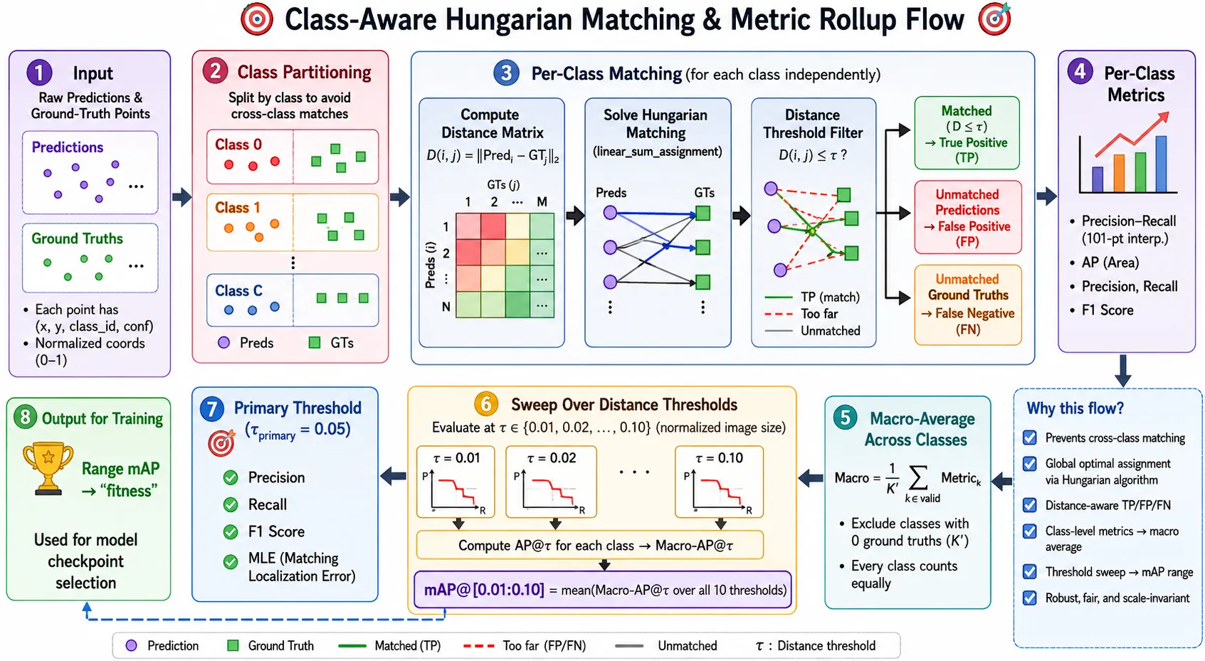
[POINT COORDINATE] mAP@d
Mean Average Precision at distance . Calculate the Area Under the Curve (AUC) for the Precision-Recall curve at a specific distance radius.
[POINT COORDINATE] mAP@d-[0.01:0.10]
The mean of mAP scores calculated at strict distance intervals (e.g., ). This is the point-based equivalent of the COCO mAP@[0.50:0.95] metric.
[POINT COORDINATE] Point localization error
For all True Positives, what is the average Euclidean distance between the predicted coordinate and the exact ground truth coordinate?
[POINT COORDINATE] Precision
Out of all points the model predicted, how many were actually correct?
[POINT COORDINATE] Recall
Out of all the ground truth points that actually exist, how many did the model successfully find?
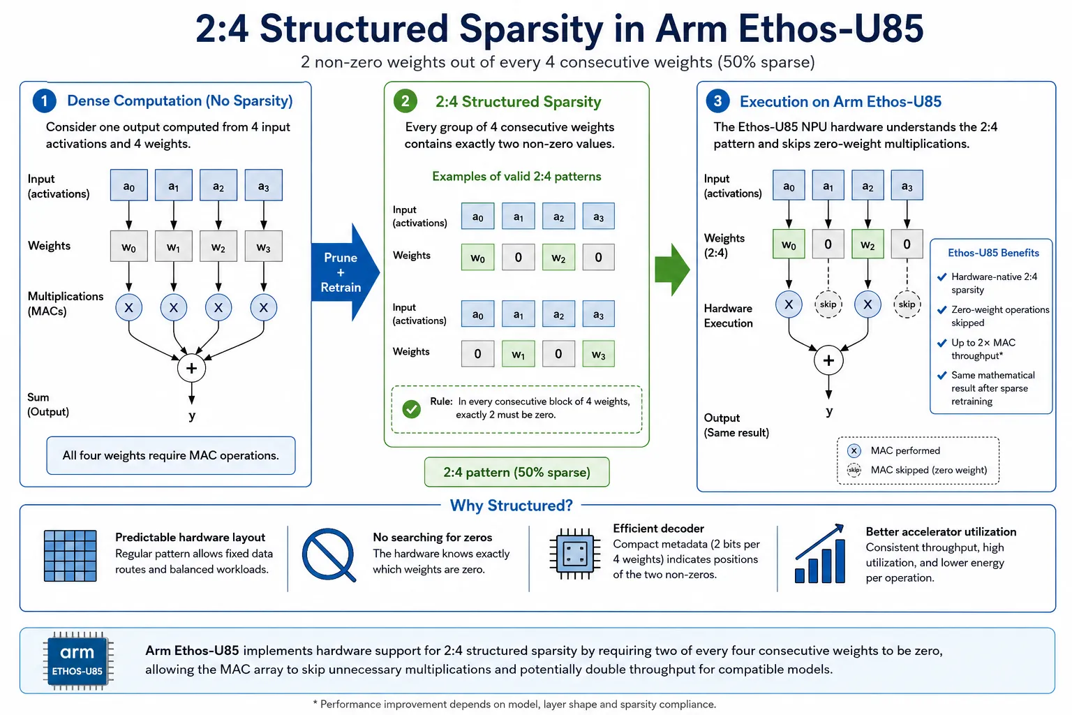
2:1 structured sparsity
F1 score
Harmonic mean of Precision and Recall. We use it when we want a single metric that balances both, especially when we have an uneven class distribution.
Inception-v3
Inception-v3 is a 48-layer deep convolutional neural network (CNN) for image classification, developed by Google in 2016 to improve accuracy while reducing computational cost.
Introduced label smoothing.
L1 Regularization (Lasso)
A method of penalizing weights proportional to their L1 norm, the sum of their absolute values (Manhattan Distance). Pushes weights to zero, encourages sparsity.
Where:
- : The final objective function to be minimized.
- : The original loss function (e.g., MSE, Cross-Entropy) measuring the error on the training data.
- (Lambda): The regularization strength hyperparameter. Controls the trade-off between fitting the data and keeping weights small.
- : The L1 norm of the weight vector.
L2 Regularization (Ridge)
A method of penalizing weights proportional to their L1 norm, the sum of their absolute values (Manhattan Distance). Pushes weights to zero, encourages sparsity.
Where:
- : The final objective function to be minimized.
- : The original loss function (e.g., MSE, Cross-Entropy) measuring the error on the training data.
- (Lambda): The regularization strength hyperparameter. Controls the trade-off between fitting the data and keeping weights small.
- : The L1 norm of the weight vector.
Language Model Samplers
| Sampler | How it works | The Flaw |
|---|---|---|
| Top-K | Keeps only the most likely tokens. | Too rigid; ignores context confidence. |
| Top-P | Keeps tokens until their cumulative probability hits . | Can let in terrible tokens if the model is confused. |
| Min-P | Sets a threshold relative to the top token’s probability (e.g., must be at least as likely as the #1 choice). | None; seamlessly adapts to both high confidence and high chaos. |
Matching Phase (Bipartite Matching)
To calculate precision and recall, we must assign predictions to ground truth points. We cannot just measure the distance of every prediction to every ground truth. We need a 1:1 mapping.
For each prediction, we find the nearest ground truth point.
If the distance is within the allowed tolerance, we consider it a match. If the ground truth point is already matched to a closer prediction, we consider the current prediction a false positive.
Any ground truth point without a match is a false negative.
| Class | Definition |
|---|---|
| True Positive (TP) | A prediction is within distance of an unmatched ground truth point. |
| False Positive (FP) | A prediction that does not fall within distance of any ground truth point, or the ground truth point is already “claimed” by a closer prediction. |
| False Negative (FN) | A ground truth point that has no prediction within distance . |
precision (metric)
You’re fishing with a net. You use a wide net, and catch 80 of 100 total fish in a lake. That’s 80% recall. But you also get 80 rocks in your net. That means 50% precision, half of the net’s contents is junk. You could use a smaller net and target one pocket of the lake where there are lots of fish and no rocks, but you might only get 20 of the fish in order to get 0 rocks. That is 20% recall and 100% precision.
recall (metric)
You’re fishing with a net. You use a wide net, and catch 80 of 100 total fish in a lake. That’s 80% recall. But you also get 80 rocks in your net. That means 50% precision, half of the net’s contents is junk. You could use a smaller net and target one pocket of the lake where there are lots of fish and no rocks, but you might only get 20 of the fish in order to get 0 rocks. That is 20% recall and 100% precision.
Also just the True Positive Rate (TPR).
Skip Connections
In classical hidden layer backprop calculations, we focused heavily on calculating gradients to update our weights, solvings . To mathematically reach a weight matrix deep in the early layers of the network, the error signal from the loss function must first survive the journey through all the intermediate activations above it.
We multiply by the weight matrix and the activation derivative at every single layer. When is , or initialized weights are small, terms multiply together and decay exponentially towards zero, causing the vanishing gradient problem.
When we add skip connections [1], we add the input as a residual:
represents the composite function of all operations. We take the input , pass it through our architecture , and add the result back to the original input.
During backpropagation, we want to pass the gradient of the loss back to . Applying the chain rule:
Now, let’s expand the local derivative based on our residual equation:
Substitute this back into the chain rule:
The first term, , represents the standard gradient flowing through the weights of the convolutional layers. In a deep network, this term might still vanish to zero.
The second term, , is same gradient from the layer above, passing completely through the + operator. Because the gradient is added rather than multiplied, the loss landscape becomes smoother.
Instead of forcing to learn a new representation of data, carries historical information forward. is now responsible for learning the residual needed to improve the current representation. If a particular layer decides it doesn’t need to learn anything new, the optimizer pushes the weights of toward zero. The output becomes .
Sparsity
Sparsity is when you force most of the weights or activations in a neural network to be zero, keeping only the most important connections. Usually you can keep 98% of the accuracy while removing most of the weights.